
Fantasy Premier League Classification Model Using Scikit Learn
A Supervised Learning Classification Model Example Using Scikit Learn
This is my attempt at producing a classification model in Python using the Scikit-Learn package. I’m going to use Fantasy Premier League player data from the 2017/18 season to create a model that will attempt to predict the position of a player given their player stats. There are four possible prediction classes: Goalkeeper, Defender, Midfielder, Forward.
Notes on the Data
The CSV file containing the player data has been preprocessed into a format compatible with Scikit-Learn. All the stats (feature) columns were numerical anyway so there were no categorical variables that needed dealing with. There is no missing data in any of the columns of the dataset.
Players could be on the field accruing stats for up to 3420 minutes (38 full matches) during the season, indeed 10 players did just that. I removed all players from the dataset who played less than 180 minutes (the equivalent of 2 full matches). That still leaves lots of players who will have played far less than others and their comparative lack of stats will no doubt impact on model performance. As this is an example rather than a model intending to have any great practical use I’ll proceed while understanding that limitation is there.
The target column ‘Position’ will need to be processed as it contains strings (GK, DF, MF, FW). As I understand it in scikit-learn the prediction classes need to be numerical values, I’ll show how to encode that column using scikit-learn LabelEncoder.
Importing our Dataset
#Import relevant packages
import numpy as np
import pandas as pd
import matplotlib.pyplot as plt
import seaborn as sns
import itertools

#Import our CSV data file as a dataframe
fpl_data = pd.read_csv('https://eddiesport.github.io/projects/FPL_final.csv', \
                       header=0, index_col=0, encoding='cp1252')

print(fpl_data.head())
print(fpl_data.info())
                        Position  Goals Scored  Assists  Clean Sheets  \
Full Name
Eldin Jakupovic               GK             0        0             0
Jeremy Pied                   DF             0        1             0
Kyle Walker Peters            DF             0        2             1
Beni Baningime                MF             0        0             0
Konstantinos Mavropanos       DF             0        0             1

                         Goals Conceded  Own Goals  Penalties Saved  \
Full Name
Eldin Jakupovic                       6          0                0
Jeremy Pied                           3          0                0
Kyle Walker Peters                    4          0                0
Beni Baningime                        2          0                0
Konstantinos Mavropanos               5          0                0

                         Penalties Missed  Yellow Cards  Red Cards  Saves  \
Full Name
Eldin Jakupovic                         0             0          0      8
Jeremy Pied                             0             0          0      0
Kyle Walker Peters                      0             0          0      0
Beni Baningime                          0             1          0      0
Konstantinos Mavropanos                 0             0          1      0

                         Bonus Points  Bonus Point System Score  Influence  \
Full Name
Eldin Jakupovic                     0                        36       67.8
Jeremy Pied                         1                        47       65.8
Kyle Walker Peters                  0                        73       70.4
Beni Baningime                      0                        20        9.4
Konstantinos Mavropanos             0                        41       52.2

                         Creativity  Threat  ICT Index
Full Name
Eldin Jakupovic                 0.0       0        6.8
Jeremy Pied                    29.9       4       10.0
Kyle Walker Peters             48.3      10       12.9
Beni Baningime                  3.8       0        1.3
Konstantinos Mavropanos         1.3       2        5.5
<class 'pandas.core.frame.DataFrame'>
Index: 441 entries, Eldin Jakupovic to Asmir Begovic
Data columns (total 17 columns):
Position                    441 non-null object
Goals Scored                441 non-null int64
Assists                     441 non-null int64
Clean Sheets                441 non-null int64
Goals Conceded              441 non-null int64
Own Goals                   441 non-null int64
Penalties Saved             441 non-null int64
Penalties Missed            441 non-null int64
Yellow Cards                441 non-null int64
Red Cards                   441 non-null int64
Saves                       441 non-null int64
Bonus Points                441 non-null int64
Bonus Point System Score    441 non-null int64
Influence                   441 non-null float64
Creativity                  441 non-null float64
Threat                      441 non-null int64
ICT Index                   441 non-null float64
dtypes: float64(3), int64(13), object(1)
memory usage: 62.0+ KB
None
We can see that the created DataFrame contains the players names as the index and 17 data columns. None of the columns appears to have missing data (as expected given its been preprocessed). The 16 numerical columns are going to be our features while the ‘Position’ column will be our target. Lets encode this column now so scikit-learn will accept it.
Encoding our Feature Column
#Using Label Encoder
from sklearn.preprocessing import LabelEncoder

#Instantiate an example of LabelEncoder
le = LabelEncoder()
#Apply to our target column
fpl_data.Position = le.fit_transform(fpl_data.Position)

#Create a dictionary to show our newly encoded key/value pairs
#The class_names variable will also be used in our visualizations later
class_names = le.classes_
values = le.transform(le.classes_)
dictionary = dict(zip(class_names, values))
print(dictionary)
{'DF': 0, 'FW': 1, 'GK': 2, 'MF': 3}
As we can see, our target classes are now numeric, with 0 representing ‘DF’, 1 for ‘FW’, etc.
Create our Feature and Target Arrays
#Create feature (X) and target (y) arrays
feature_cols = ['Goals Scored', 'Assists', 'Clean Sheets', 'Goals Conceded', 'Own Goals', 'Penalties Saved', \
                'Penalties Missed', 'Yellow Cards', 'Red Cards', 'Saves', 'Bonus Points', 'Bonus Point System Score', \
                'Influence', 'Creativity', 'Threat', 'ICT Index']

X = fpl_data.loc[:, feature_cols]
print(X.shape)

y = fpl_data.Position
print(y.shape)

print(y.value_counts())
(441, 16)
(441,)
3    182
0    159
1     66
2     34
Name: Position, dtype: int64
Something to note is the class imbalance of our target variable, for example we have far more midfielders (182) than goalkeepers (34). This is something to bear in mind when looking at the results of testing our model later.
A Visualization of our Feature Columns
I should have done some graphical EDA earlier to see if relationships between our feature columns existed. As I’ve just separated the feature columns out I’ll produce a correlation matrix of all our 16 variables. Given there are quite a lot of variables I’ll then create a heatmap of the result.
#Create a show a correlation matrix of the feature columns
corr_mat = X.corr()

#Visualize this matrix using Seaborns heatmap function
sns.heatmap(corr_mat)
plt.title('Feature Columns Correlation Heatmap')
plt.show()
plt.clf()
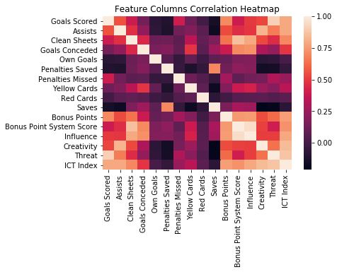
Unsurprisingly there are a range of relationships here, ‘Goals Scored’ and ‘Threat’ are highly correlated, while ‘Penalities Saved’ and ‘Creativity’ are not. There’s certainly enough going on that one should hope a useful classification model could be trained using the data, so lets continue!
Scaling our Data
If the various columns of data cover differing ranges (from min to max values in each column) then we should look into rescaling our data. Lets take a look.
#Quick look at the DataFrames column data statistical details
print(fpl_data.describe())
         Position  Goals Scored     Assists  Clean Sheets  Goals Conceded  \
count  441.000000    441.000000  441.000000    441.000000      441.000000
mean     1.541950      2.235828    2.047619      5.773243       25.090703
std      1.341195      3.784980    2.813926      4.104688       14.925601
min      0.000000      0.000000    0.000000      0.000000        0.000000
25%      0.000000      0.000000    0.000000      3.000000       13.000000
50%      1.000000      1.000000    1.000000      5.000000       24.000000
75%      3.000000      3.000000    3.000000      9.000000       34.000000
max      3.000000     32.000000   18.000000     19.000000       63.000000

        Own Goals  Penalties Saved  Penalties Missed  Yellow Cards  \
count  441.000000       441.000000        441.000000    441.000000
mean     0.068027         0.047619          0.054422      2.612245
std      0.301357         0.277980          0.280802      2.329989
min      0.000000         0.000000          0.000000      0.000000
25%      0.000000         0.000000          0.000000      1.000000
50%      0.000000         0.000000          0.000000      2.000000
75%      0.000000         0.000000          0.000000      4.000000
max      4.000000         3.000000          3.000000     11.000000

        Red Cards       Saves  Bonus Points  Bonus Point System Score  \
count  441.000000  441.000000    441.000000                441.000000
mean     0.088435    4.863946      5.467120                323.800454
std      0.299814   20.584738      5.960814                201.358017
min      0.000000    0.000000      0.000000                 11.000000
25%      0.000000    0.000000      0.000000                167.000000
50%      0.000000    0.000000      4.000000                305.000000
75%      0.000000    0.000000      9.000000                470.000000
max      2.000000  145.000000     31.000000                913.000000

         Influence   Creativity       Threat   ICT Index
count   441.000000   441.000000   441.000000  441.000000
mean    390.402268   252.426531   268.795918   91.133560
std     261.424449   268.366338   321.296859   71.471795
min       8.800000     0.000000     0.000000    1.300000
25%     181.800000    59.400000    55.000000   36.800000
50%     353.800000   164.700000   150.000000   76.900000
75%     550.400000   340.700000   361.000000  120.600000
max    1496.200000  1744.200000  2355.000000  454.400000
We can see a large variation in ranges, eg, ‘Penalties Saved’ ranges from 0-3, while Threat ranges from 0-2355. This suggests we should include scale our data within the model. I’ll do this using Standardization.
What Type of Classification Model To Use?
Scikit-learn gives lots of choices, I’m going to use a K-Nearest Neighbors (k-NN) classifier here. To be more thorough one could try many models and see which performs better given your metrics of choice.
Create a Pipeline Object
I’m going to standardize my data, then apply the k-NN model. This is two seperate steps, so I’ll put them in a pipeline!
#Import required scikit-learn modules
from sklearn.model_selection import train_test_split, GridSearchCV
from sklearn.neighbors import KNeighborsClassifier
from sklearn.preprocessing import StandardScaler
from sklearn.pipeline import Pipeline

#Set up the pipeline steps
steps = [('scaler', StandardScaler()),
         ('knn', KNeighborsClassifier())]

#Create the pipeline object
pipeline = Pipeline(steps)
Hyperparameter Tuning
We are going to tune the n_neighbors parameter of our k-NN classifier. To do this I’ll create a range of ‘n_neighbors’ to try. I’ll use 1-20 here.
#Define parameter grid for K neighbors search
k_range = np.arange(1, 21)
parameters = {'knn__n_neighbors': k_range}
Train Test Split
Lets create our training and test sets. Add in a random state for repeatability of results.
#Create training and test (hold out) sets
X_train, X_test, y_train, y_test = train_test_split(X, y, test_size = 0.25, random_state=42, stratify=y)
Instantiate a GridSearch Object
Lets add our pipeline and parameters to a gridsearch object. Cross validation is set to 3 subsets by default, I’ll change it to 5 here. The result of this will be, for bettor or worse, our model.
#Instantiate GridSearch object.
fpl_model = GridSearchCV(pipeline, parameters, cv=5)
Train and Test our Model, show Model Metrics
#Fit model to training set
fpl_model.fit(X_train, y_train)

#Predict labels of the test data
y_pred = fpl_model.predict(X_test)

#Compute and print metrics
from sklearn.metrics import classification_report, confusion_matrix

#Print accuracy, classification report and the best model parameters used
print('Accuracy: {}'.format(fpl_model.score(X_test, y_test)))
print(classification_report(y_test, y_pred))
print("Tuned Model Parameters: {}".format(fpl_model.best_params_))
Accuracy: 0.7297297297297297
             precision    recall  f1-score   support

          0       0.69      0.78      0.73        40
          1       0.79      0.65      0.71        17
          2       1.00      0.88      0.93         8
          3       0.71      0.70      0.70        46

avg / total       0.74      0.73      0.73       111

Tuned Model Parameters: {'knn__n_neighbors': 3}
An accuracy score of 0.7298. Well its a lot better than guessing that everyone was a Midfielder (the most numerous class), that would have yielded an accuracy score of 0.41, so our model is definitely working. From our hyperparameter tuning we can see the optimum number of ‘n_neighbors’ in this case was 3.
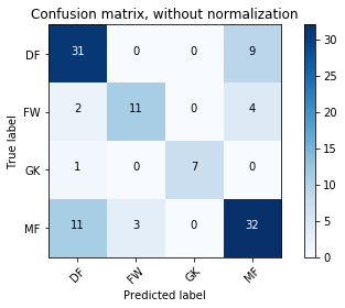
Lets look at another model metric, the confusion matrix. The following code that defines a function for visualizing a confusion matrix is not mine, its taken from the scikit-learn docs. The first example is not normalized, the second one is. Normalizing is a good idea here because of the class imbalance we mentioned earlier.
#Function to visualize the confusion matrix
def plot_confusion_matrix(cm, classes,
                          normalize=False,
                          title='Confusion matrix',
                          cmap=plt.cm.Blues):
    """
    This function prints and plots the confusion matrix.
    Normalization can be applied by setting `normalize=True`.
    """
    if normalize:
        cm = cm.astype('float') / cm.sum(axis=1)[:, np.newaxis]
        print("Normalized confusion matrix")
    else:
        print('Confusion matrix, without normalization')

    print(cm)

    plt.imshow(cm, interpolation='nearest', cmap=cmap)
    plt.title(title)
    plt.colorbar()
    tick_marks = np.arange(len(classes))
    plt.xticks(tick_marks, classes, rotation=45)
    plt.yticks(tick_marks, classes)

    fmt = '.2f' if normalize else 'd'
    thresh = cm.max() / 2.
    for i, j in itertools.product(range(cm.shape[0]), range(cm.shape[1])):
        plt.text(j, i, format(cm[i, j], fmt),
                 horizontalalignment="center",
                 color="white" if cm[i, j] > thresh else "black")

    plt.ylabel('True label')
    plt.xlabel('Predicted label')
    plt.tight_layout()
# Compute confusion matrix
cnf_matrix = confusion_matrix(y_test, y_pred)

#Plot non-normalized confusion matrix
plt.figure()
plot_confusion_matrix(cnf_matrix, classes=class_names,
                      title='Confusion matrix, without normalization')

#Plot normalized confusion matrix
plt.figure()
plot_confusion_matrix(cnf_matrix, classes=class_names, normalize=True,
                      title='Normalized confusion matrix')

plt.show()
Confusion matrix, without normalization
[[31  0  0  9]
 [ 2 11  0  4]
 [ 1  0  7  0]
 [11  3  0 32]]
Normalized confusion matrix
[[ 0.775       0.          0.          0.225     ]
 [ 0.11764706  0.64705882  0.          0.23529412]
 [ 0.125       0.          0.875       0.        ]
 [ 0.23913043  0.06521739  0.          0.69565217]]


<matplotlib.figure.Figure at 0xc08beb8>
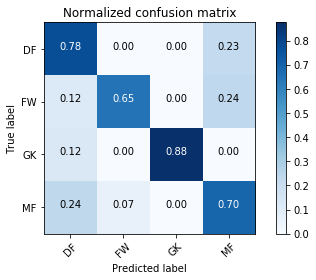
We can see from the normalized confusion matrix that the model was good at predicting goalkeepers on the test set, less good at predicting forwards.
If you like the created model and want to run it again in future it would be wise to save it as a file (I’m not going to do that here though).
Using our Model for Prediction
I don’t have an unused data set to try the model on but I will apply it here back to the original dataset and see what we get.
#Use model to predict on full dataset
model_result = fpl_model.predict(X)

#Compute and print metrics
print('Accuracy: {}'.format(fpl_model.score(X, y)))
print(classification_report(y, model_result))

#Compute confusion matrix on whole data set
cnf_matrix = confusion_matrix(y, model_result)

#Plot non-normalized confusion matrix
plt.figure()
plot_confusion_matrix(cnf_matrix, classes=class_names,
                      title='Confusion matrix, without normalization')

#Plot normalized confusion matrix
plt.figure()
plot_confusion_matrix(cnf_matrix, classes=class_names, normalize=True,
                      title='Normalized confusion matrix')

plt.show()
Accuracy: 0.8276643990929705
precision recall f1-score support
0 0.79 0.87 0.83 159
1 0.86 0.74 0.80 66
2 1.00 0.94 0.97 34
3 0.83 0.80 0.81 182
avg / total 0.83 0.83 0.83 441
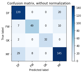
Confusion matrix, without normalization
[[139 0 0 20]
[ 7 49 0 10]
[ 2 0 32 0]
[ 29 8 0 145]]
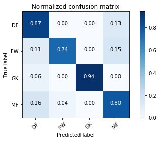
Normalized confusion matrix
[[ 0.87421384 0. 0. 0.12578616]
[ 0.10606061 0.74242424 0. 0.15151515]
[ 0.05882353 0. 0.94117647 0. ]
[ 0.15934066 0.04395604 0. 0.7967033 ]]
Thoughts
What, if anything, can we ascertain from these results? We can see from the confusion matrix on the full dataset that 8 midfielders were misclassified by our model as forwards. For fantasy players these misclassifications could provide a potentially interesting insight, as midfielders who act like forwards are likely to be valuable in fantasy terms. Lets see who these 8 players actually are.
To begin I’ll add the predictions back into the original dataset by adding a ‘Results’ column.
#Add model result to full dataset
fpl_data['Results'] = model_result
print(fpl_data.info())
<class 'pandas.core.frame.DataFrame'>
Index: 441 entries, Eldin Jakupovic to Asmir Begovic
Data columns (total 18 columns):
Position                    441 non-null int64
Goals Scored                441 non-null int64
Assists                     441 non-null int64
Clean Sheets                441 non-null int64
Goals Conceded              441 non-null int64
Own Goals                   441 non-null int64
Penalties Saved             441 non-null int64
Penalties Missed            441 non-null int64
Yellow Cards                441 non-null int64
Red Cards                   441 non-null int64
Saves                       441 non-null int64
Bonus Points                441 non-null int64
Bonus Point System Score    441 non-null int64
Influence                   441 non-null float64
Creativity                  441 non-null float64
Threat                      441 non-null int64
ICT Index                   441 non-null float64
Results                     441 non-null int64
dtypes: float64(3), int64(15)
memory usage: 85.5+ KB
None
Our new position column has been added and looks good. I’ll now do some DataFrame slicing and (just for clarity here) create a new DataFrame (fpl_wrong) that contains all the players our model misclassified. From that new DataFrame I’ll select the midfielders (class 3) who the model predicted as forwards (class 1).
#Create a new DataFrame of players who have been misclassified by the model
fpl_wrong = fpl_data.loc[fpl_data['Position'] != fpl_data['Results']]

#Select midfielders classified by our model as forwards
print(fpl_wrong[(fpl_wrong['Position'] == 3) & (fpl_wrong['Results'] == 1)])
                          Position  Goals Scored  Assists  Clean Sheets  \
Full Name
Gnegneri Yaya Toure              3             0        2             0
Adam Lallana                     3             0        0             1
Junior Stanislas                 3             5        3             2
Eric Maxim Choupo Moting         3             5        5             5
James McArthur                   3             5        2             7
Wilfried Zaha                    3             9        7            10
Richarlison de Andrade           3             5        8             8
Mohamed Salah                    3            32       12            15

                          Goals Conceded  Own Goals  Penalties Saved  \
Full Name
Gnegneri Yaya Toure                    2          0                0
Adam Lallana                           1          0                0
Junior Stanislas                      22          0                0
Eric Maxim Choupo Moting              45          0                0
James McArthur                        35          0                0
Wilfried Zaha                         31          0                0
Richarlison de Andrade                54          0                0
Mohamed Salah                         29          0                0

                          Penalties Missed  Yellow Cards  Red Cards  Saves  \
Full Name
Gnegneri Yaya Toure                      0             1          0      0
Adam Lallana                             0             1          0      0
Junior Stanislas                         0             1          0      0
Eric Maxim Choupo Moting                 0             3          0      0
James McArthur                           0             5          0      0
Wilfried Zaha                            0             5          0      0
Richarlison de Andrade                   0             4          0      0
Mohamed Salah                            1             1          0      0

                          Bonus Points  Bonus Point System Score  Influence  \
Full Name
Gnegneri Yaya Toure                  0                        99      105.0
Adam Lallana                         0                        37       32.6
Junior Stanislas                     7                       285      394.8
Eric Maxim Choupo Moting             9                       341      505.6
James McArthur                       9                       416      490.6
Wilfried Zaha                        8                       404      668.0
Richarlison de Andrade               4                       304      497.0
Mohamed Salah                       26                       881     1496.2

                          Creativity  Threat  ICT Index  Results
Full Name
Gnegneri Yaya Toure            122.6      72       29.8        1
Adam Lallana                   113.4     128       27.3        1
Junior Stanislas               377.2     483      125.1        1
Eric Maxim Choupo Moting       327.5     851      168.1        1
James McArthur                 333.0     566      138.9        1
Wilfried Zaha                  716.9    1125      251.0        1
Richarlison de Andrade         384.7    1217      209.3        1
Mohamed Salah                  942.5    2109      454.4        1
We have our 8 players. They include Mo Salah, the Premier League top scorer in the 2017/18 season. This is promising, if any player should be misclassified its Salah, a midfielder who scores 30+ goals a season. Another player is Zaha, in this current (18/19) seasons fantasy game he is no longer listed as a midfielder but as a forward, so this misclassification is also perfectly understandable. There is definitely scope here for checking this list between seasons to try and find potential value players for the following years game.
We’ll thats our k-NN Classification model! Its not perfect, we knew given the data limitations described in the intro it couldn’t be, but it still worked pretty well and could even be used to provide some insight into the fantasy Premier League game.
Leave a Comment